Plotting DSP data¶

KFR can generate plots for a univector or another sized numeric container. The plotting functions write a Python script and run it with python, falling back to python3 when necessary. The script uses the repository's dspplot package to draw the figure. This is a convenient development and documentation tool, not a real-time plotting API.

Include <kfr/io.hpp> (or <kfr/all.hpp>) to use the plotting functions.

Prerequisites¶

Install Python and ensure that either python or python3 is available on PATH. The renderer requires NumPy, SciPy, and Matplotlib. From the repository root, install the project requirements with:

python3 -m pip install -r requirements.txt

Alternatively, install just the plotting dependencies:

python3 -m pip install numpy scipy matplotlib

The generated Python script locates KFR's in-tree dspplot module relative to the script. When using an installed copy of KFR rather than a source checkout, make that module available to Python separately, for example by installing the dspplot package from the repository's dspplot directory.

Plotting numeric data¶

plot_show opens a plot window. plot_save saves an SVG instead. Both functions copy the input samples into a generated Python list, so use a reasonably sized numeric container such as univector. Non-finite floating-point values are written as zero.

For numeric data, the default figure has a sample-domain plot and an FFT-derived magnitude response. The magnitude plot uses the first half of an FFT whose size is at least the input length and padwidth (1024 by default). It is displayed in dB with a floor of \(-300\ \mathrm{dB}\). The default frequency axis is 10 Hz to \(Fs/2\), where Fs defaults to 48000 Hz.

univector<float> data = { 0.0f, 1.0f, 0.5f, 0.0f, -0.5f };

plot_show("signal", data,
          "title='Signal', Fs=48000, log_freq=True, padwidth=8192");

The third argument is inserted directly as Python keyword arguments. It is therefore Python syntax, not a C++ options object. Use single quotes inside the C++ string for a title, as in the example.

Example: plotting a window¶

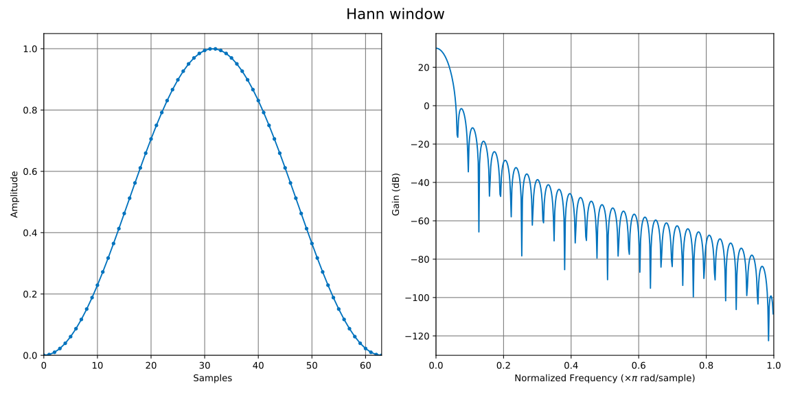
This Hann-window example shows the samples as points and its normalized-frequency magnitude response. It uses the same output generated for the Window functions examples.

1
2
3
4
5
6

const std::string options = "freqresp=True, dots=True, padwidth=1024, "
                            "log_freq=False, horizontal=False, normalized_freq=True";
univector<fbase, 64> output;

output = window_hann(output.size());
plot_save("window_hann", output, options + ", title='Hann window'");

Saving a plot¶

univector<float> data = { 0.0f, 1.0f, 0.5f, 0.0f, -0.5f };
plot_save("signal", data,
          "title='Signal', Fs=48000, log_freq=True, padwidth=8192");

plot_save writes signal.py to the process's current working directory and asks the renderer to save the image as ../svg/signal.svg relative to that directory. Create the destination directory before running the program. Do not pass file=... in the options string: plot_save supplies the output path itself.

Plotting filter responses¶

Pass filter coefficients or an impulse response as numeric data. For an FIR filter with centred, odd-length coefficients, phasearg='auto' removes the linear phase due to the coefficient centre. For a response delayed by a known number of samples, pass that delay as a numeric phasearg instead.

const auto sections = iir_params{ biquad_lowpass<float>(1000.0f / 48000.0f, 0.707f) };
univector<float, 1024> response = iir(unitimpulse(), sections);

plot_save("lowpass_response", response,
          "title='Low-pass response', Fs=48000, phaseresp=True, "
          "log_freq=True, freq_dB_lim=(-160, 10), padwidth=8192");

Set Fs whenever the response was designed for a specific sample rate so that the frequency scale is correct. log_freq=True selects a logarithmic frequency axis; normalized_freq=True instead displays a \(0\) to \(1\) axis in units of \(\times\pi\) rad/sample. freq_dB_lim=(low, high) fixes the magnitude range. Set div_by_N=True to divide FFT bins by the sample count before converting to dB, which is useful when comparing spectra of signals with different lengths.

The most useful plotting options are:

Plotting WAV files¶

Passing a std::string or const char* file name to plot_show selects the WAV/spectrogram path rather than the numeric-data path:

plot_save("recording", "recording.wav",
          "title='Recording', segmentsize=1024, overlap=8");

This path is intended for WAV files and produces a spectrogram. It is separate from KFR's general audio decoder support; see Reading and Writing Audio Files to load, process, or save other supported audio formats. For numeric data, spectrogram=True also routes the renderer to this spectrogram view. segmentsize, overlap, vmin, vmax, and normalize set its analysis and display parameters.

Troubleshooting¶

• If no window appears or no SVG is written, first run the generated .py script from the current working directory to see Python's error output.
• Confirm that python or python3 selects the interpreter where the required packages were installed. KFR tries python first.
• Python plotting is unavailable on mobile and WebAssembly targets. The plotting functions report failures to standard error and return without rendering a plot.
• The name argument becomes the generated script file name and, for plot_save, part of the SVG path. Use a simple file-name-safe value.

See also¶

• FIR filters
• IIR filters
• Reading and Writing Audio Files